Getting Started
Emanuel Rodriguez
2021-09-20
CDECRetrieve.RmdInstall
You can install CDECRetrieve the usual way,
# for stable version
install.packages("CDECRetrieve")

# for development version
devtools::install_github("flowwest/CDECRetrieve")
Intro
The goal for CDECRetrieve is to create a workflow for R users using CDEC data, we believe that a well defined workflow is easier to automate and less prone to error (or easier to catch errors). In order to do this we create “services” out of different endpoints available through the CDEC site. A lot ideas in developing the package came from using dataRetrieval from USGS and the NOAA CDO api.
Exploring Locations
We start by first exploring locations of interest. The CDEC site provides a web form with a lot of options,
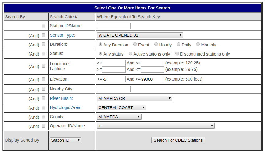
cdec station search
The pakcage exposes this functionallity through cdec_stations(). Although it doesn’t (currently) map all options in the web form it does so for the most used, namely, station id, nearby city, river basin, hydro area and county. At least one of the parameters must be supplied, and combination of these can be supplied to refine the search.
library(CDECRetrieve)

cdec_stations(station_id = "kwk") # return metadata for KWK
#> # A tibble: 1 x 9
#>   station_id name  river_basin county longitude latitude elevation operator
#>   <chr>      <chr> <chr>       <chr>      <dbl>    <dbl>     <int> <chr>
#> 1 kwk        sacr~ sacramento~ shasta     -122.     40.6       596 US Geol~
#> # ... with 1 more variable: state <chr>

# show all locations near san francisco, this returns a set of
# CDEC station that are near San Francisco
cdec_stations(nearby_city = "san francisco")
#> # A tibble: 3 x 9
#>   station_id name  river_basin county longitude latitude elevation operator
#>   <chr>      <chr> <chr>       <chr>      <dbl>    <dbl>     <int> <chr>
#> 1 cx2        dail~ sf bay      san f~     -122.     37.8         0 CA Dept~
#> 2 sfn        san ~ sf bay      san f~     -122.     37.8       150 Nationa~
#> 3 ggt        gold~ sf bay      san f~     -122.     37.8         0 Nationa~
#> # ... with 1 more variable: state <chr>

# show all location in the sf bay river basin
cdec_stations(river_basin = "sf bay")
#> # A tibble: 25 x 9
#>    station_id name  river_basin county longitude latitude elevation operator
#>    <chr>      <chr> <chr>       <chr>      <dbl>    <dbl> <chr>     <chr>
#>  1 hml        moun~ sf bay      santa~     -122.     37.3 4,206     Nationa~
#>  2 okm        oakl~ sf bay      alame~     -122.     37.8 30        Nationa~
#>  3 snn        san ~ sf bay      san m~     -122.     37.6 456       San Fra~
#>  4 cx2        dail~ sf bay      san f~     -122.     37.8 0         CA Dept~
#>  5 sfn        san ~ sf bay      san f~     -122.     37.8 150       Nationa~
#>  6 sff        san ~ sf bay      san m~     -122.     37.6 8         Nationa~
#>  7 spb        san ~ sf bay      contr~     -122.     37.9 330       East Ba~
#>  8 rwc        redw~ sf bay      none ~    -1000.    100.  31        .None S~
#>  9 vsb        vall~ sf bay      alame~     -122.     37.6 635       CA Dept~
#> 10 lfy        lafa~ sf bay      contr~     -122.     37.9 465       East Ba~
#> # ... with 15 more rows, and 1 more variable: state <chr>

# show all station in Tehama county
cdec_stations(county = "tehama")
#> # A tibble: 46 x 9
#>    station_id name  river_basin county longitude latitude elevation operator
#>    <chr>      <chr> <chr>       <chr>      <dbl>    <dbl> <chr>     <chr>
#>  1 bnd        sacr~ sacramento~ tehama     -122.     40.3 286       US Geol~
#>  2 blb        blac~ stony cr    tehama     -122.     39.8 426       US Army~
#>  3 ctn        cott~ cottonwood~ tehama     -123.     40.3 3,400     US Bure~
#>  4 dch        deer~ sacramento~ tehama     -121.     40.3 50        CA Dept~
#>  5 sh1        shee~ sacramento~ tehama     -123.     39.5 6,500     US Army~
#>  6 vno        sacr~ sacramento~ tehama     -122.     39.9 185       CA Dept~
#>  7 bsf        sacr~ sacramento~ tehama     -122.     40.4 360       US Bure~
#>  8 bat        batt~ sacramento~ tehama     -122.     40.4 200       USGS/DWR
#>  9 sad        sadd~ cottonwood~ tehama     -123.     40.2 3,850     CA Dept~
#> 10 ec1        eagl~ battle cre~ tehama     -122.     40.4 1,591     Pacific~
#> # ... with 36 more rows, and 1 more variable: state <chr>
Since we are simply exploring for locations of interest, it may be useful to map these for visual inspection. CDECRetrieve provides a simple function to do exactly this map_stations().
library(magrittr)
library(leaflet)

cdec_stations(county = "tehama") %>%
  map_stations()
The same can be done with leaflet functions
d <- cdec_stations(county = "tehama")
leaflet(d) %>%
  addTiles() %>%
  addCircleMarkers(label=~station_id) #psk is way off here
Exploring Datasets within a Station
After exploring stations in a desired location. We can start focusing on the datasets available at the locations.
station <- "sha"
cdec_datasets("sha")
#> # A tibble: 21 x 6
#>    sensor_number sensor_name         sensor_units duration start      end
#>            <int> <chr>               <chr>        <chr>    <date>     <date>
#>  1             2 precipitation accu~ inches       daily    2003-10-01 2020-12-10
#>  2             2 precipitation accu~ inches       monthly  1953-10-01 2020-12-10
#>  3             6 reservoir elevation feet         daily    1985-01-01 2020-12-10
#>  4             6 reservoir elevation feet         hourly   1993-12-09 2020-12-10
#>  5             8 full natural flow   cfs          daily    1987-05-31 2020-12-10
#>  6            15 reservoir storage   af           daily    1985-01-01 2020-12-10
#>  7            15 reservoir storage   af           hourly   1994-06-24 2020-12-10
#>  8            15 reservoir storage   af           monthly  1953-10-01 2020-12-10
#>  9            22 reservoir storage ~ af           daily    1993-10-03 2020-12-10
#> 10            23 reservoir outflow   cfs          daily    1987-01-05 2020-12-10
#> # ... with 11 more rows
Since all of these functions return a tidy dataframe we can make use of the dplyr to filter, mutate and explore. Here we look for datasets in Shasta that report a storage
library(magrittr)

cdec_datasets("sha") %>%
  dplyr::filter(grepl("storage", sensor_name))
#> # A tibble: 5 x 6
#>   sensor_number sensor_name          sensor_units duration start      end
#>           <int> <chr>                <chr>        <chr>    <date>     <date>
#> 1            15 reservoir storage    af           daily    1985-01-01 2020-12-10
#> 2            15 reservoir storage    af           hourly   1994-06-24 2020-12-10
#> 3            15 reservoir storage    af           monthly  1953-10-01 2020-12-10
#> 4            22 reservoir storage c~ af           daily    1993-10-03 2020-12-10
#> 5            94 reservoir top conse~ af           daily    2000-10-24 2020-12-10
Take note of the sensor number, and duration, these will be needed for querying data in the next section.
Query Data
Now that we have a location, parameter of interest and duration we can start to query for actual data.
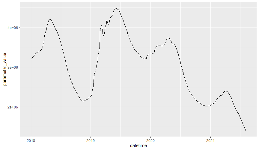
sha_storage_daily <- cdec_query(station = "sha", sensor_num = "15",
                                dur_code = "d", start_date = "2018-01-01",
                                end_date = Sys.Date())

sha_storage_daily
#> # A tibble: 1,075 x 5
#>    agency_cd location_id datetime            parameter_cd parameter_value
#>    <chr>     <chr>       <dttm>              <chr>                  <dbl>
#>  1 CDEC      SHA         2018-01-01 00:00:00 15                   3203249
#>  2 CDEC      SHA         2018-01-02 00:00:00 15                   3202064
#>  3 CDEC      SHA         2018-01-03 00:00:00 15                   3203723
#>  4 CDEC      SHA         2018-01-04 00:00:00 15                   3206566
#>  5 CDEC      SHA         2018-01-05 00:00:00 15                   3210358
#>  6 CDEC      SHA         2018-01-06 00:00:00 15                   3215097
#>  7 CDEC      SHA         2018-01-07 00:00:00 15                   3217003
#>  8 CDEC      SHA         2018-01-08 00:00:00 15                   3229391
#>  9 CDEC      SHA         2018-01-09 00:00:00 15                   3237014
#> 10 CDEC      SHA         2018-01-10 00:00:00 15                   3242032
#> # ... with 1,065 more rows
Once again the the data is in a tidy form.