DRAFT
This article documents a set of solutions for different types of queries carried out on output from 2d hec-ras models.
Most of these recipes will make use of dplyr, purrr as well as ggplot2 and plotly for visualizations. Make sure these are installed before running examples.
Read and Explore
library(hecr)
h <- hec_file("../inst/examples/LowerDeerCreek_2018.p10.hdf")

print(h)

# A hec object----
# Plan File: LowerDeerCreek_2018.p10
# Plan Name: Existing_LidarCalib_20180830
# Geom Name: LowerDeerCreek_2018.g13
# Out Inteval: 15MIN
Glimpse at HDF Structure
tree(h)

# *Group:  Event Conditions
#   |
#   -- Unsteady
#
# *Group:  Geometry
#   |
#   -- 2D Flow Area Break Lines
#   |
#   -- 2D Flow Areas
#   |
#   -- Boundary Condition Lines
#   |
#   -- Land Cover (Manning's n)
#   |
#   -- River Bank Lines
#   |
#   -- River Edge Lines
#   |
#   -- River Flow Paths
#   |
#   -- River Stationing
#   |
#   -- Structures
#
# *Group:  Plan Data
#   |
#   -- Plan Information
#   |
#   -- Plan Parameters
#
# *Group:  Results
#   |
#   -- Summary
#   |
#   -- Unsteady
You can glimpse deeper into the structure by passing the depth value to tree(). This is a nice utility to have, but for in depth exploration we recommend using HDFView available from the HDF Group.
hdf5r
The HDF backend for the package is provided through hdf5r. A user is able to explore using the hdf5r API by exposing the HDF5 object:
# h is still the 'hec-file' object from above
hdf_obj <- h$object

print(hdf_obj)

# Class: H5File
# Filename: /home/emanuel/Projects/hecr/inst/examples/LowerDeerCreek_2018.p10.hdf
# Access type: H5F_ACC_RDONLY
# Attributes: File Type, Units System, File Version, Projection
# Listing:
#              name  obj_type dataset.dims dataset.type_class
#  Event Conditions H5I_GROUP         <NA>               <NA>
#          Geometry H5I_GROUP         <NA>               <NA>
#         Plan Data H5I_GROUP         <NA>               <NA>
#           Results H5I_GROUP         <NA>               <NA>
Learn more about hdf5r here
The rest of this article focuses on common queries.
One plan one coordinate
The most basic query is one coordinate and one plan. There is no additional manipulation of hec_two() to make this query happen.
coord <- c(6570468.12123, 1881034.38489)
data <- hec_two(h, coord)

glimpse(data)

# Observations: 97
# Variables: 8
# $ datetime         <dttm> 2018-02-07 00:00:00, 2018-02-...
# $ plan_id          <chr> "Existing_LidarCalib_20180830"...
# $ plan_file        <chr> "LowerDeerCreek_2018.p10", "Lo...
# $ time_series_type <chr> "Water Surface", "Water Surfac...
# $ hdf_cell_index   <dbl> 445700, 445700, 445700, 445700...
# $ xin              <dbl> 1, 1, 1, 1, 1, 1, 1, 1, 1, 1, ...
# $ yin              <dbl> 2, 2, 2, 2, 2, 2, 2, 2, 2, 2, ...
# $ values           <dbl> 196.020980834961, 196.02098083...
The structure of the data is as follows:
| Column Nmae | Description |
|---|---|
| datetime | a datatime object with date and time of record |
| plan_id | a string with the name of the plan |
| plan_file | a string with the name of file queried from |
| time_series_type | the time series that was queried |
| hdf_cell_index | the cell index from the hdf file that was chosen for the coordinate |
| xin | the corresponding x-coordinate supplied |
| yin | the corresponding y-coordinate supplied |
| values | the value of the time series |
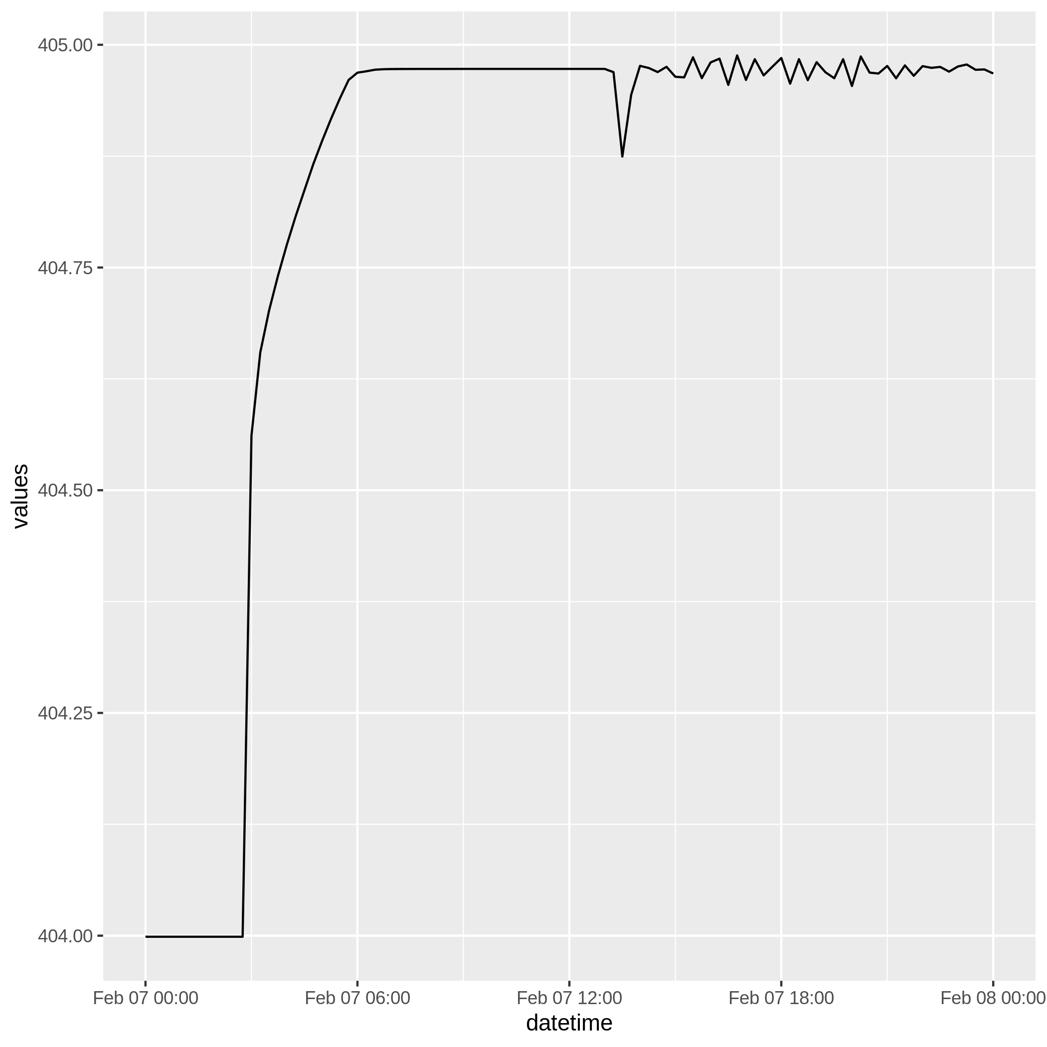
We can plot this data using ggplot2

one plan
One plan multiple coordinates
To query multiple coordinates out of the hdf file, simply provide a matrix, or an even length vector of coordinates. The matrix must be mx2 here m is the number of coordinates and 2 is the x and y coordinates (in that order). There is no limit on m. The other option is a vector of pairs of coordinates, therefore of even length. We currently support vector for quick queries and testing but a sophisicated script should be supplying a matrix as input.
# define a vector of coordinates
coords_vs <- c(6570468.12123,   1881034.38489,
            6570186.03222,  1880216.19001,
            6570167.9381,   1879820.21836,
            6570141.81282,  1879703.42988,
            6570114.02745,  1879601.38152,
            6570108.19281,  1879582.69751,
            6569969.28791,  1879291.13936
)

# you can also supply a matrix
coords_m <- matrix(coords_vs, ncol=2, byrow = TRUE)

data <- hec_two(h, coords_m)

dplyr::glimpse(data)

# Observations: 679
# Variables: 8
# $ datetime         <dttm> 2018-02-07 00:00:00, 2018-02-07 00:15:00, 2018-02-07 00:30:00, ...
# $ plan_id          <chr> "Existing_LidarCalib_20180830", "Existing_LidarCalib_20180830", ...
# $ plan_file        <chr> "LowerDeerCreek_2018.p10", "LowerDeerCreek_2018.p10", "LowerDeer...
# $ time_series_type <chr> "Water Surface", "Water Surface", "Water Surface", "Water Surfac...
# $ hdf_cell_index   <dbl> 391410, 391410, 391410, 391410, 391410, 391410, 391410, 391410, ...
# $ xin              <dbl> 6570468.12123, 6570468.12123, 6570468.12123, 6570468.12123, 6570...
# $ yin              <dbl> 1881034.38489, 1881034.38489, 1881034.38489, 1881034.38489, 1881...
# $ values           <dbl> 403.998809814453, 403.998809814453, 403.998809814453, 403.998809...
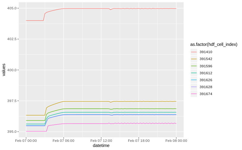
When you query multiple coordinates, the “hdf_cell_index” becomes an importnat attribute, it maps the input coordinate (that you supplied) to the corresponding cell in the model that hecr determined to be the closest. You can use this attrbute to, group by, color and other “group” operations.
Here we plot the time series based on these inputs, and color by the cell index. Note that the cell index a numeric and thus needs to casted to factor or character for ggplot to properly display these are different time series.

multiple coords
One Plan, mutiple coodinates for one timestamp (Profile Line)
With the optional time stamp parameter, you can fix the time portion of query to a desired stamp and query values for a large number of coordinates. Although you could query all data then perform a filter to a time stamp (which you can totally do), passing in the time stamp allows you to save a lot memory resources since the package will only read in the time stamp desired straight from the hdf file (using hdf5r).
coords_m

tstamp <- "2018-02-07 01:15:00"

data <- hec_two(f, coords_m, time_stamp = tstamp)

glimpse(data)

# Observations: 7
# Variables: 8
# $ datetime         <dttm> 2018-02-07 01:15:00, 2018-02-07 01:15:00, 2018-02-07 01:15:00, ...
# $ plan_id          <chr> "Existing_LidarCalib_20180830", "Existing_LidarCalib_20180830", ...
# $ plan_file        <chr> "LowerDeerCreek_2018.p10", "LowerDeerCreek_2018.p10", "LowerDeer...
# $ time_series_type <chr> "Water Surface", "Water Surface", "Water Surface", "Water Surfac...
# $ hdf_cell_index   <dbl> 391410, 391542, 391596, 391612, 391626, 391628, 391674
# $ xin              <dbl> 6570468.12123, 6570186.03222, 6570167.93810, 6570141.81282, 6570...
# $ yin              <dbl> 1881034.38489, 1880216.19001, 1879820.21836, 1879703.42988, 1879...
# $ values           <dbl> 403.998809814453, 396.334991455078, 395.906250000000, 395.625000...
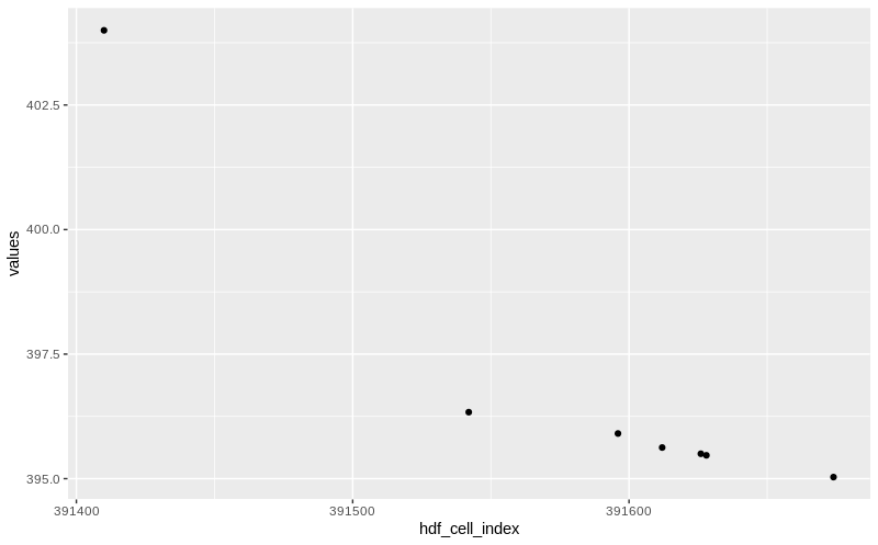
As expected the output now only has 7 observations, one for each coordinate, each reporting the value observed at the time specified.
Here we plot this:
data %>%
  ggplot(aes(hdf_cell_index, values)) + geom_point()
profile line