Adobe Streamflow Model

library(adobeCreekData)
library(tidyverse)
library(lubridate)
library(mgcv)

Introdcuction

Give a little intro about the the purpose of the model and the overall results.

Data

The data being used to develop this model is USGS streamflow data. The following gages were used:

• Highland Creek - 11449010 (1966-1977)
• Kelsey Creek - 11449500 (1970-present)
• Adobe Creek - 11448500 (1954-1978)

The Highland Creek gage is below Highland dam, the Adobe Creek gage is above the Adobe Creek dam. All this data is bundled within this data package, more information for each is available with:

?adobeCreekData::kelsey_creek_flow

In order to calculate Adobe Creek after the Highland Creek junction we summed up the two flows.

adobe_creek_downstream <- 
  adobeCreekData::adobe_creek_flow %>% 
  left_join(adobeCreekData::highland_creek_flow, by=c("date" = "date"), 
            suffix = c("_adobe", "_highland")) %>% 
  select(date, flow_cfs_highland, flow_cfs_adobe) %>% 
  mutate(adobe_downstream_cfs = flow_cfs_highland + flow_cfs_adobe) %>% 
  filter(!is.na(adobe_downstream_cfs))

This resulted in the following streamflow

adobe_creek_downstream %>% 
  filter(year(date) == 1975, month(date) %in% 2:8) %>% 
  ggplot() + 
  geom_line(aes(date, adobe_downstream_cfs, color="Adobe Downstream")) + 
  geom_line(aes(date, flow_cfs_highland, color="Highland Creek")) + 
  geom_line(aes(date, flow_cfs_adobe, color="Adobe Creek")) + 
  labs(x = "Date", y = "Flow (cfs)", color="")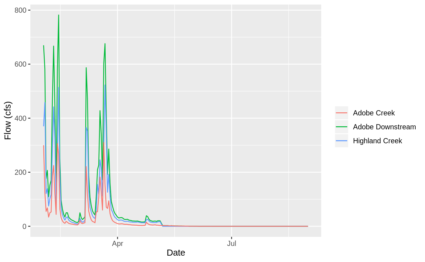

This is the streamflow data we will use to develop this model.

Modeling Approach

There is clear correlation between the two creeks, it appears that we can capture this relatioship with some form of linear regression. In this section we explore several alternatives of regression and select the optimal one.

flow_data <- adobe_creek_downstream %>% 
  left_join(kelsey_creek_flow, by=c("date" = "date")) %>% 
  select(date, flow_cfs_highland, 
         flow_cfs_adobe, 
         adobe_downstream_cfs, 
         kelsey_cfs = flow_cfs) %>% 
  filter(!is.na(kelsey_cfs))

training_data <- flow_data %>% filter(year(date) != 1975)
test_data <- flow_data %>% filter(year(date) == 1975)

training_data %>% 
  ggplot(aes(kelsey_cfs, adobe_downstream_cfs)) + 
  geom_point(alpha=0.4) + 
  labs(x = "Kelsey Creek Flow (cfs", y = "Adobe Creek Flow (cfs)")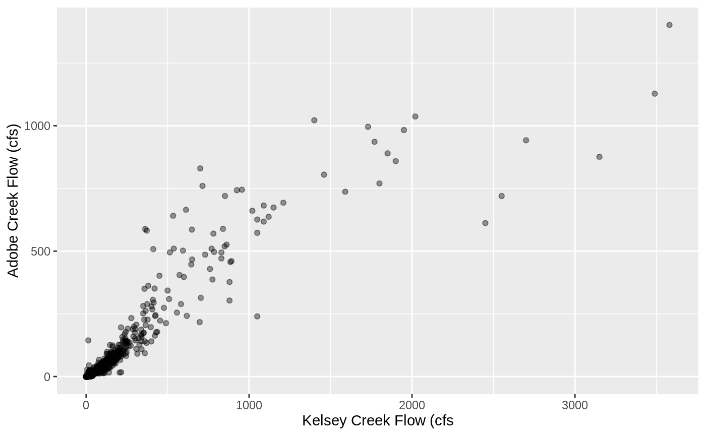

Linear Regression

As we can see

training_data %>% 
  ggplot(aes(kelsey_cfs, adobe_downstream_cfs)) + 
  geom_point(alpha=0.4) + 
  geom_smooth(method = "lm", formula = y ~ x ) + 
  labs(x = "Kelsey Creek Flow (cfs", y = "Adobe Creek Flow (cfs)")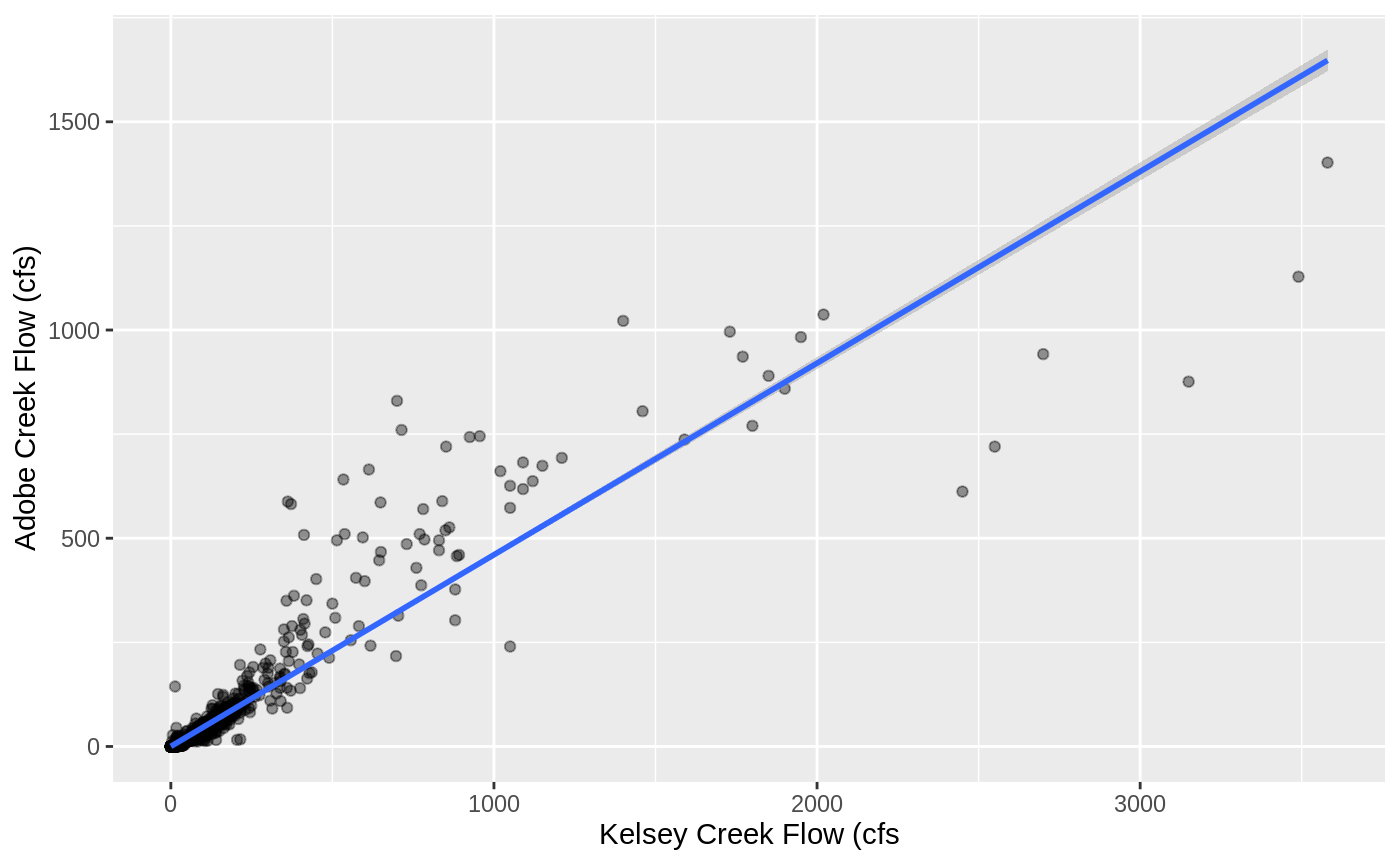 

lin_reg_model <- lm(adobe_downstream_cfs ~ kelsey_cfs, data = training_data)
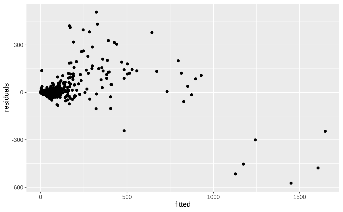
lin_reg_evaluation <- tibble(
  date = training_data$date, 
  actuals = training_data$adobe_downstream_cfs, 
  fitted = fitted(lin_reg_model), 
  residuals = residuals(lin_reg_model)
)

lin_reg_evaluation %>% 
  ggplot(aes(fitted, residuals)) + geom_point()

Generalized Additive Model

gam_model <- gam(adobe_downstream_cfs ~ s(kelsey_cfs, bs = "cs"), data = training_data)

Model Evaluation

Results

Conclusion