Groundwater Trends

Introduction

In this article I explore groundwater elevation trends, we are interested in exploring elevation differences by water year. We will focus only on wells that have had recent measurements. Ultimately we would like to develop confidence intervals for elevation change based on the characteristics of a water year.

Groundwater Well Selection

We will focus on wells where a groundwater elevation was reported for 2018. This results in 23 candiate wells for analysis. This number will be smaller as we seek to make comparison across years.

Elevation Change

Here I look at the change of elevation in one year. Here are the assumptions and requirements for this analysis:

site code must have recent data to at least 2018
only subsequent years of data will be taken into account
when attaching water year types to the fall difference we will always use the water year for September. For example even though the difference is from November 1980 to November 1981, the water year associated with this difference will be 1980.

How the difference is calcualted

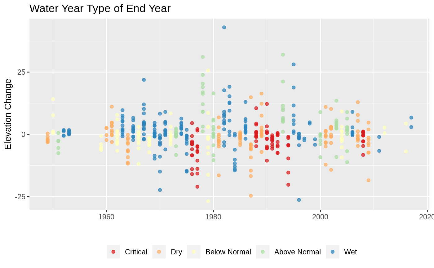
The difference is calculated by subtracting the “start year” (smaller of the years) from the “end year”. This means that a positive value indicates elevation increase and a negative value indicates elevation decrease. When looking at the plot, a point on 1980 shows the difference between 1979 and 1980. Lastly this subtraction is done on each well, so when looking the plot a single point shows the difference between two years at an individual site code. We can see the spread of the difference values for a given year by focusing on one year on the x-axis and observing the range of values on the y-axis.

Elevation Change Time Series By Water Year Type

Here I color code the points by the water year type of the end year. That is, when looking at the year 1980 the value indicates the difference between wells from 1979 to 1980 but the color shows the water year type for 1980. No obvious patterns appear in the data. I instead switch to looking at the distribution of elvetaion changes for each of the water year types.

Distribution of Elevation Changes

With the water years attached we can do some statistics using these as categorical variables. We are mainly interested in significant differences in elevation change as a result of the water year types. In order to do so we need to have enough samples from the each of the water year types.

Year Type Representation

Year Type	Total	Percent of data (%)
Critical	82	15
Dry	121	22
Below Normal	86	15
Above Normal	82	15
Wet	184	33

Most of the data is from either a Wet or Dry year, but we do have enough samples each of the other water years.

Significant Differences between year types

In this section I analyze the distribution of elevation change between the water year types. In particular we are interested in answering the following questions:

Is there a significant difference between dry years (dry, critical) and wet years (Abobe Normal, Wet).
Does the water year type of the previous affect the elevation change? If so how much?
Given a water year type is there a range of expected elevation change we can anticipate?
For all of the above, if we can’t answer then question now, what additional data would we need to do so?

Several assumptions must be met before we develop statistical test

Question 1: Significant Differences between Year Types

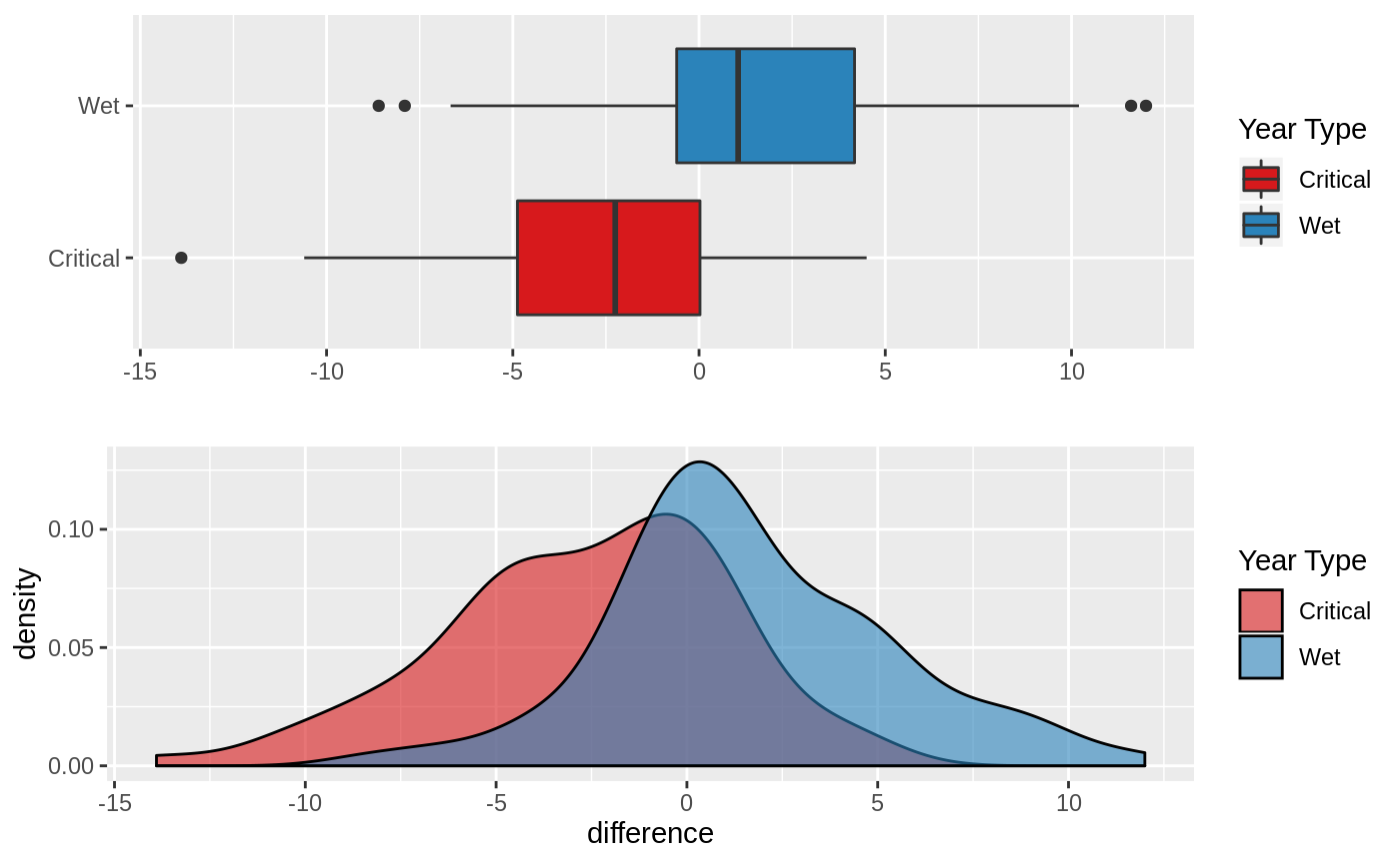
In this section I explore the differences between the elevation changes across the different water year types. We want to be able to state whether the distributions shown in the boxplots below are significantly different from one another.

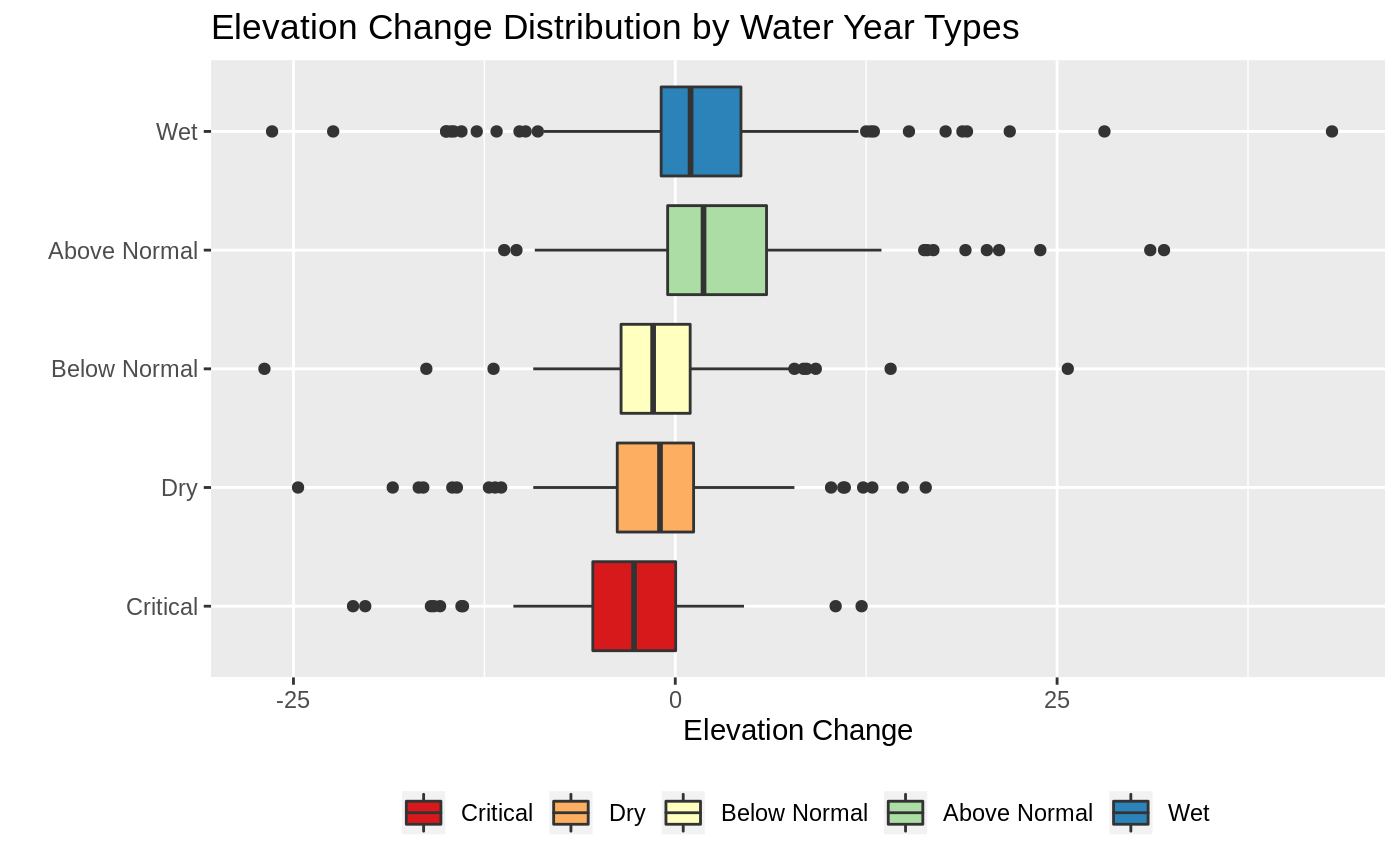
The plan here is to use two sample test to check for significant differences. There are several assumtpions that need to be satisfied in order for this analysis to be valid, we check these below.

Assumption checks

Normality

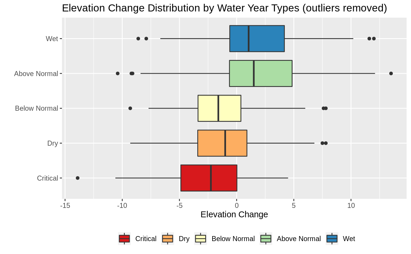
From the boxplot we can see that the elevation change across all of the water year types are at least symmetrical. There might be some issues from the detected outliers. I apply the Shapiro test to check for normality before and after removing outliers.

Water Year Type	Total Sample	Total Outliers Detected	Test with Removed Outliers	Test on Full Sample
Critical	82	8	TRUE	FALSE
Dry	121	16	TRUE	FALSE
Below Normal	86	8	TRUE	FALSE
Above Normal	82	10	TRUE	FALSE
Wet	184	22	FALSE	FALSE

From the above results we can see that none of the elevation change distrubtions (that include the outliers) can be assumed to be normally distributed. When we remove the outliers, counted under the Total Outliers Detected column, then most of the Water Year types can be considered normally distribute, with the exception of the Above Normal elevation changes.

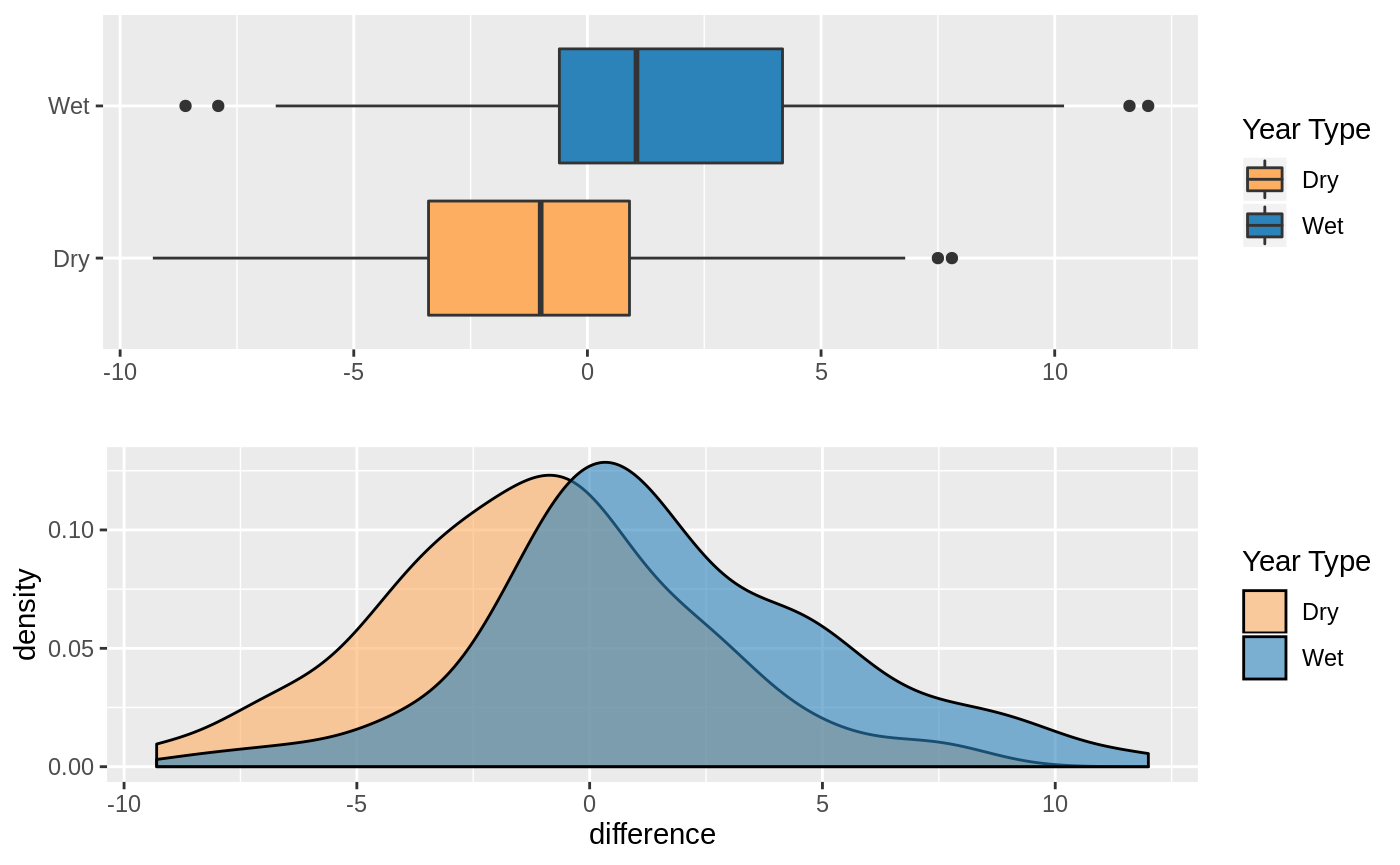
Wet Year vs Dry Year

Wet Year vs Critical Year

Wet or Above Normal vs Critical, Dry or Below Normal

Question 2: Previous Year Type effect on Elevation Changes

#> [1] 38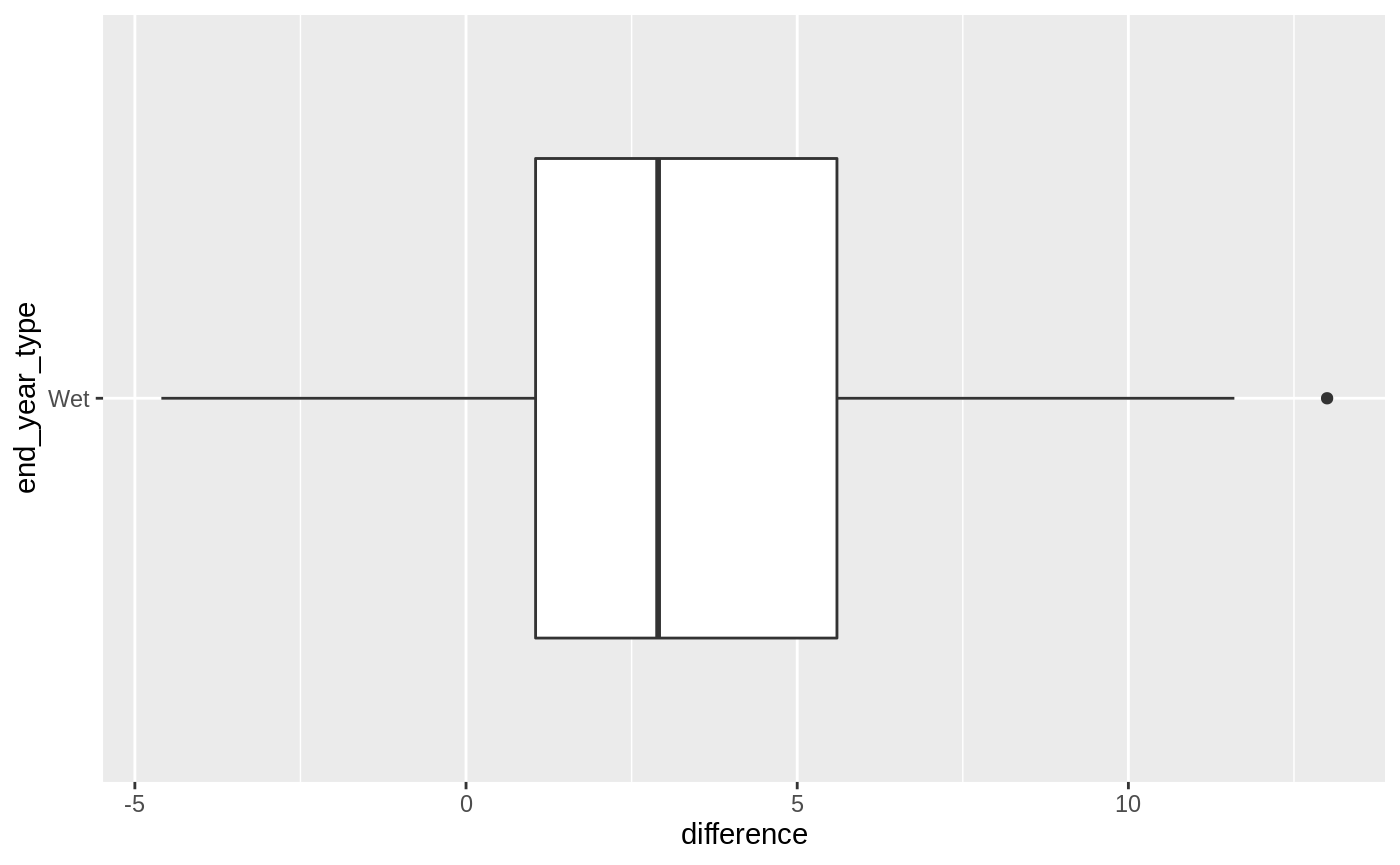

#> 
#>  Shapiro-Wilk normality test
#> 
#> data:  dry_types_to_wet[!dry_types_to_wet$is_outlier_for_dry_to_wet,     ]$difference
#> W = 0.98713, p-value = 0.9334
#> 
#>  Shapiro-Wilk normality test
#> 
#> data:  wet_vals
#> W = 0.98145, p-value = 0.0286
#> 
#>  One Sample t-test
#> 
#> data:  dry_types_to_wet[!dry_types_to_wet$is_outlier_for_dry_to_wet,     ]$difference
#> t = 5.3732, df = 37, p-value = 2.216e-06
#> alternative hypothesis: true mean is greater than 0
#> 95 percent confidence interval:
#>  2.318021      Inf
#> sample estimates:
#> mean of x 
#>  3.378947
#> 
#>  One Sample t-test
#> 
#> data:  wet_vals
#> t = 5.5598, df = 161, p-value = 5.498e-08
#> alternative hypothesis: true mean is greater than 0
#> 95 percent confidence interval:
#>  1.139388      Inf
#> sample estimates:
#> mean of x 
#>  1.622037
#> 
#>  Welch Two Sample t-test
#> 
#> data:  wet_vals and dry_types_to_wet[!dry_types_to_wet$is_outlier_for_dry_to_wet, wet_vals and     ]$difference
#> t = -2.5344, df = 54.066, p-value = 0.01419
#> alternative hypothesis: true difference in means is not equal to 0
#> 95 percent confidence interval:
#>  -3.1467079 -0.3671128
#> sample estimates:
#> mean of x mean of y 
#>  1.622037  3.378947