Statistical Model Development, Training, and Prediction

Introduction

We are currently developing and refining a statistical model to predict flow-to-suitable-habitat-area relationships for stream reaches in the Sacramento-San Joaquin Basin, based on a variety of widely-available geospatial and hydrologic variables. Predictor variable data collection is detailed in the Predictor Variables article.

This statistical model method was developed for predicting rearing habitat area versus flow at the comid scale.

It is also applied for spawning habitat area, given training data generated using different habitat suitability indices (see Habitat Training Data), with additional post-model filters required to eliminate areas that are non-suitable due to substrate (see Spawning Extents).

Raw outputs from this method are then ready to be scaled based on hydrology and duration requirements (see Duration Analysis) and/or aggregated at the river or watershed level (see Watershed Aggregation).

Model Development

General Model Form

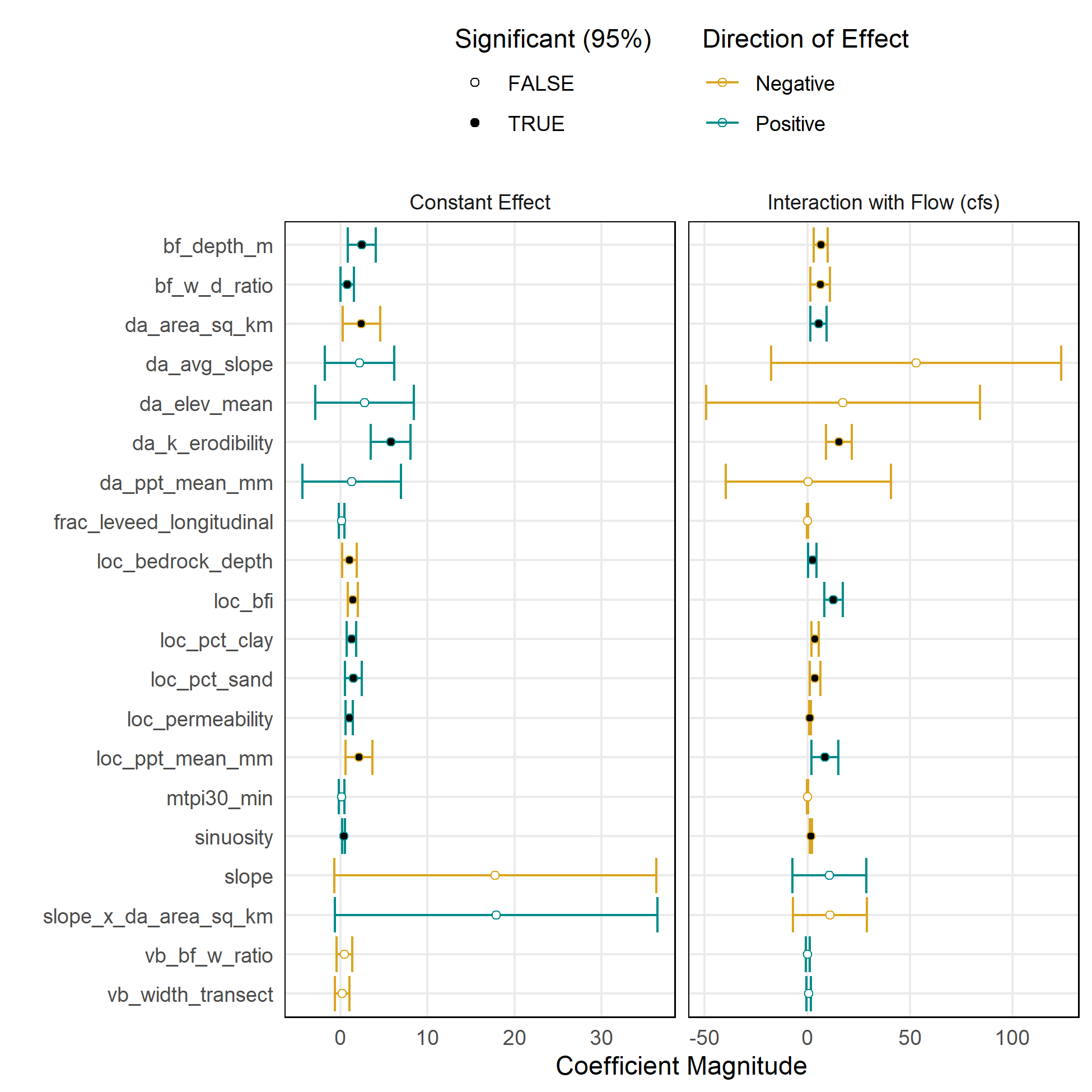
In practice, suitable habitat area is modeled as a function of flow, the suite of predictor variables, and the interactions between each predictor variable and flow. As applied in a linear regression model, the general functional form for the model is as follows. The use of the interaction terms allows the model to estimate not only the average effect of each predictor variable on suitable area, but also the effect of each predictor variable on the flow-to-suitable-area relationship.

$\mathbf{h} = \alpha + \beta\mathbf{q} + \pmb{\gamma}\mathbf{X} + \pmb{\delta}\mathbf{q}\mathbf{X} + \epsilon$

$\mathbf{h}$ = suitable habitat area, WUA per linear ft (response variable)
$\mathbf{q}$ = streamflow (cfs)
$\mathbf{X}$ = matrix of predictor variables (slope, drainage area, etc.)
$\alpha$ = estimated intercept
$\beta$ = estimated coefficient on flow (i.e. constant effect of flow on habitat)
$\pmb{\gamma}$ = estimated coefficients of predictor variables (i.e., constant effect of each predictor on habitat)
$\pmb{\delta}$ = estimated coefficients of interactions (i.e., effect of each predictor on the flow-to-habitat relationship)
$\epsilon$ = error term

Expressed without using matrix notation, the model estimate for each NHD ComID reach $i$ and flow $q$ is…

${SuitableHabitatArea}_{i,q} = \alpha + \beta{Flow}_{q} + \gamma_1{Slope}_{i} + \delta_1{Flow}_{q}{Slope}_{i} + \gamma_2{DrainageArea}_{i} + \delta_2{Flow}_{q}{DrainageArea}_{i} + ... + \epsilon$

… and so on for all other predictor variables with estimated coefficients $\gamma_3$ , $\delta_3$ , $\gamma_4$ , $\delta_4$ , etc.

Transformations and Weights

We originally log-transformed the habitat, flow, and predictor variables for three reasons: (a) to limit the effect of extreme values; (b) to align with typical hydrologic conventions of using power series models; and (c) for interpretability because log-log model coefficients represent elasticities (“percent change in y per percent change in x). Because some predictor variables include values less than or equal to zero, the log transformation was replaced with a variation on the inverse hyperbolic sine (asinh) transformation. Because $\mathrm{asinh}(x) = \ln(x + \sqrt{x^2+1})$ , this transformation behaves like a log transformation for positive values ( $\mathrm{asinh}(x) \rightarrow \ln(2x) \text{ as } x \rightarrow \infty$ ) but remains defined for zero values and has a comparable, mirrored shape for negative values.

Additionally, all predictor variables were centered and scaled after transformations were applied.

The length (linear ft) of each reach (comid) was applied as a case weight. Reaches vary substantially in length from several feet to 26 miles, with a mean length of 1.2 miles. Weighting the estimate by linear ft allows longer reaches to have greater influence on the model and makes the somewhat arbitrary comid delineations less relevant.

Flow Variable

Training flow data are resampled to a regular sequence of flows that is evenly spaced on a logarithmic axis:

interp_flows <- habistat::seq_log10(50, 15000, 0.05, snap=100)

Model Versions Tested

Two forms of the model were tested, discussed in sequence in the following sections.

Model Version 1: Habitat Area/LF vs Flow

This is the simplest and most straightforward version of the model.

Habitat variable: Suitable habitat area (WUA) per linear ft, aka “effective habitat width”

Flow variable: Flow (cfs)

Predictor variables:

Reach characteristics: slope, bankfull depth, bankfull width-depth ratio, baseflow index, % clay, % sand, permeability, depth to bedrock, mean annual precipitation, MTPI (topographic position index), valley bottom width, valley bottom-bankfull width ratio, fractional levee confinement, channel sinuosity

Catchment characteristics: drainage area, mean elevation, mean annual precipitation, avg erodibility, avg slope, avg NDVI

Transformations:

Inverse hyperbolic sine

Interaction between slope and drainage area

Center and scale all predictors

Model forms: Linear regression; Random forest regression

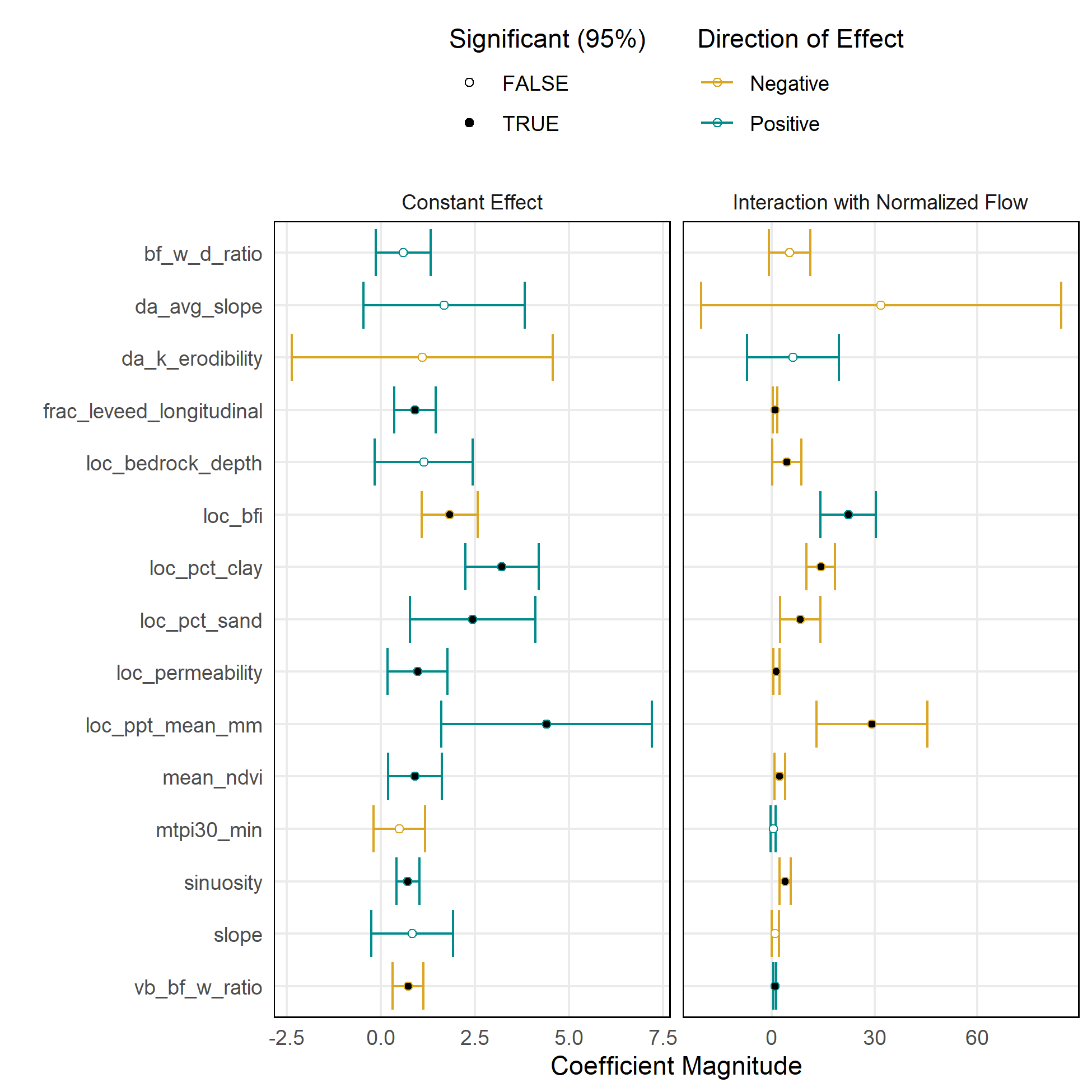
Model Version 2: Normalized Habitat Area/LF vs Normalized Flow

This model is a variation on Version 1. It is intended to deal with the problem of differing ranges of flows across training datasets on account of the differing sizes of the river systems.

A scalar was defined for each reach (comid), representing the magnitude of flow in the watershed. A product of the drainage area and mean annual precipitation with units of million acre feet (Maf), this value represents the average quantity of water input into the reach’s catchment in a year:

${Scalar [\mathrm{Maf}]} = 10^{-6} \times {DA [\mathrm{ac}]} \times {MAP [\mathrm{ft}]}$

The habitat and flow variables are multiplied by this scalar prior to prediction, then divided by the scalar after prediction.

Habitat variable: Suitable habitat area (WUA) per linear ft normalized by DA*MAP

Flow variable: Flow (cfs) normalized by DA*MAP

Predictor variables:

Reach characteristics: slope, ~~bankfull depth~~, bankfull width-depth ratio, baseflow index, % clay, % sand, permeability, depth to bedrock, ~~mean annual precipitation~~, MTPI (topographic position index), valley bottom width, valley bottom-bankfull width ratio, fractional levee confinement, channel sinuosity

Catchment characteristics: drainage area, mean elevation, mean annual precipitation, avg erodibility, avg slope, avg NDVI

Transformations:

Inverse hyperbolic sine

~~Interaction between slope and drainage area~~

Center and scale all predictors

Model forms: Linear regression; Random forest regression

Compared to Version 1, the normalized Version 2 model creates flow-to-suitable-area curves that are more strongly proportional to the size of the river.

Ensemble Model

The ensemble model is the average of the output of the Version 1 and Version 2 models for each unique combination of comid and flow.

Exploratory Linear Regression

Linear regression was useful for exploring the effects of predictor variables and testing different model forms. However, the collinearity between variables and the limitations on the functional shape of relationships were limitations.

Model Version 1: Scale-Dependent	Model Version 2: Scale-Normalized

Random Forest Regression Model

Random Forest Regression is a decision tree based machine learning alternative to linear regression. The model specifications are essentially identical to the linear regression formulations previously discussed. Unlike linear regression, there is no constraint on the functional form of the flow-to-habitat relationship or the effects of predictor variables. Random forest models are fit using the ranger package via the tidymodels framework.

Train/Test Split: Flowlines (comids) and their associated training data are split into training and testing datasets at a 75% training/25% testing random split, stratified by river and hydrologic class.
IHS Transformation: As described in the section above, all continuous numeric variables are transformed using the transformation $x' = \text{asinh}(100 \cdot x / 2)$ . Variables that represent proportions or ratios are not transformed. The response variable is also transformed.
DA/MAP Normalization: For the “scale-normalized” model, all variables are divided by the ${DA}*{MAP}$ scaling factor described above.
Interaction: Any predictor variables included in the model are also included as interactions with flow: $(x' \cdot Q)$ .
Feature Selection: The training dataset is used for feature selection, i.e., identifying the set of predictor variables to be used in the prediction. We iteratively test versions of the model with and without each predictor variable. Predictor variables selected for inclusion are those that improve model fit (decrease RMSE) when they are included relative to when they are excluded.
Parameter Tuning: Random forest model parameters are tuned using 10-fold cross-validation with the training dataset. Tuned parameters are the number of trees (trees), number of predictors that will be randomly sampled at each split when creating the tree models (mtry), and the minimum number of data points in a node that are required for the node to be split further (min_n).
Prediction: Once a final tuned model has been selected, the full dataset of flowlines (comids) and their attributes are input, once for each flow along a a regular log sequence of flows matching the interp_flows sequence described above. Predictions are run for all comids; filters are applied after the fact.
Inverse IHS Transformation: Transformed variables and the final output are reverse-transformed using $x = \text{sinh}(x') \cdot 2 / 100$ .
Inverse DA/MAP Normalization: For the “scale-normalized” model, normalization is reversed by multiplying the result by the ${DA}*{MAP}$ scaling factor described above.

Results

The trained statistical model can now be used to predict flow-to-suitable-area relationships for other streams within the study area. While the statistical model will produce predictions for any stream with valid predictor data, the validity and trustworthiness of predictions will depend on those streams’ similarity to the training dataset. As training datasets are currently limited to foothill alluvial systems on major tributary streams, only these should be considered valid.

Maddee Rubenson & Skyler Lewis

2024-10-23